1D series for kinetics:

This is a simple routine to acquire a series of 1D spectra with defined delays
It is useful for monitoring peak heights as time progresses during a reaction for example
The setup is general for any nucleus you might be observing
The final result is stored into a pseudo 2D file such that all the data is together.

Data Acquisition

*Setup your 1D expt as you normally would. This works for any 1D actually (31P, 19F etc). eg) for 1D 1H:

rpar h1.bbo all (read in 1d proton)

rpar h1_es.bbo all (use this instead if water suppression is needed; else skip)

lockdisp (open lock display window)
rsh shims.bbo (read in the latest shim files i've created)
lock (select the appropriate solvent for locking)
wobb (tune the probe)

acqu (acquisition window)

tune the probe using either the screen or the bars on preamp box next to magnet. If you need a reminder please ask us.
stop (ends tune/wobb routine)
return (exit out of acqu window back into normal 1d viewer)

now shim Z1, Z2, Z1, Z2, Z1, Z2 and push STDBY when done.
rga (set receiver gain automatically, wait a minute until it finishes)
kinetic_2d (this loads in the AU program 'kinetic_2d', be sure to answer the questions as they pop up)

kinetic_water (use this instead if you are running the h1_es.bbo experiment; else skip)

(write down the number of expts, and the delays between the experiments you've defined)
expt (this is the total time of the kinetic run as well. You can divide this by the number of 1Ds to figure delays between runs too)
zg (this will start the series of 1D acquisitions)

Data Processing

xf2 (Fourier transforms in F2 dimension only)
click the manual phase button if needed and select a row to phase. all 1Ds should then phase correctly.
the data can be processed in topspin thru the T1/T2 processing routine or on software of your choosing.
rser(12) then efp (Read slice 12 from 2D for 1D processing. OK to run this command while acquiring)

MNova_Processing

iNMR_Processing

iNMR_Download

To convert the processed 2D file into an ascii/text file please type 2dtxt - The file is saved in the current expno as "2d.txt"
Here is a copy of the AU code: 2dtxt.c

Manual Processing on the NMR or Linux OS

Copy the scripts one level up from the nmrdata folder containing the 'ser' file. scripts
If on the 400 just copy in like: cp /opt/topspin/nmrapps/scripts/kin_scripts.tar .
Now extract files: tar xvf kin_scripts.tar
Here is the link to the data processed with this tutorial for practicing if you like: practice_set

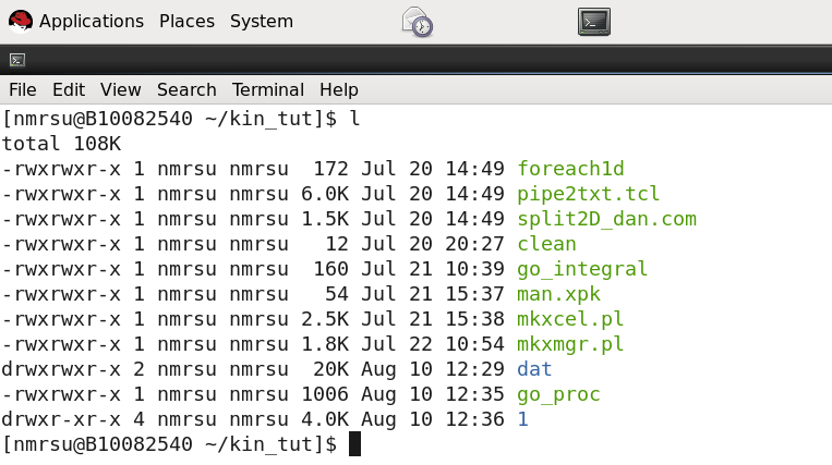
Inside your nmr data dir you should see a list of files now: ls -lrt

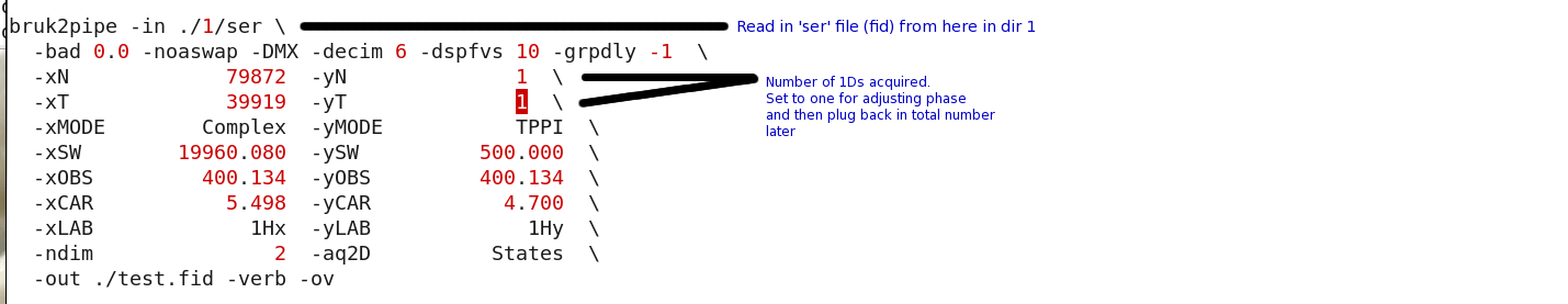
where dir '1' contains the fid/ser file. note the dir number here is whatever you designated the expno as during edc in topspin

change into dir 1 (or whatever the dir number is) - cd 1
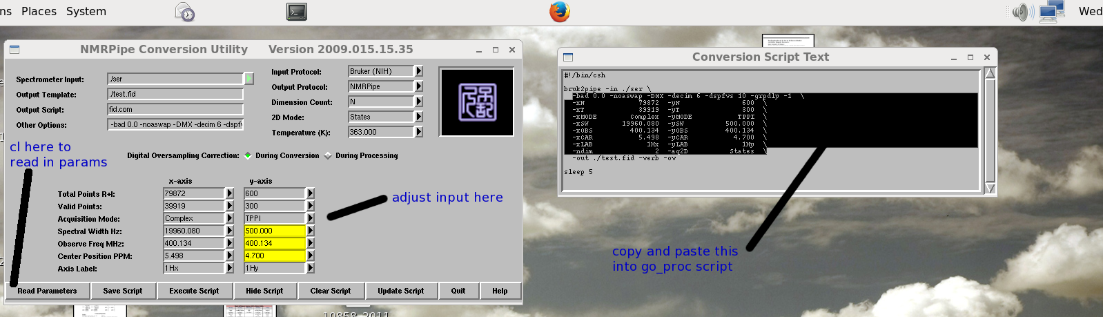
launch the bruker conversion program - bruker

Screens pop up where you read in the parameters etc or see:
D - nmrDraw is a popular NMR Viewing software thru the NIH

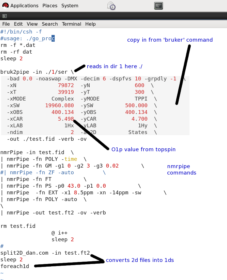
Copy in the highlighted info above into the go_proc script: gedit go_proc

The go_proc script is a master file which 1) converts the bruker to nmrPipe format and 2) processes the data using nmrPipe. Note it also later converts spectra into 1D files as we started with a 2D file. The 1D files named 001.dat etc will also be in XY text format already where X=ppm and Y=Intensity.

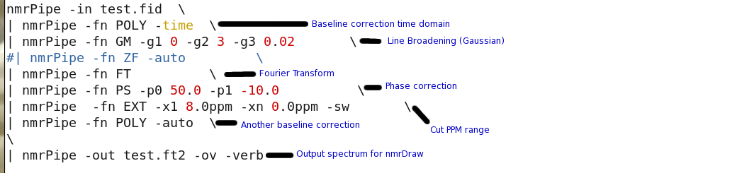
The above was a full process routine with 600 1Ds having been acquired. Lets step back and just process the first spectrum in the series so we can set the phasing correctly in nmrDraw. To process the 1st fid gedit go_proc such that:

Lets also look at how the meaning of the nmrPipe commands as well

rerun go_proc - ./go_proc
change into dir ./dat - cd dat
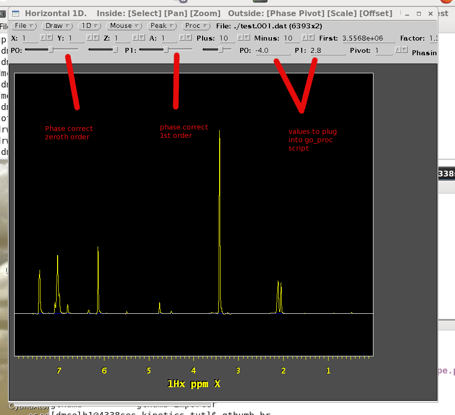
launch nmrDraw - D
read in file test.001.dat thru the pull downs.

The nmrDraw viewer opens. Now use the sliders to adjust the phase. When phased add these numbers into the -PS values in the 'go_proc' script. I like to actually set the nmrPipe phasing values to zero 1st and then just plug in the correct values determined here instead of adding them in.

edit in new phases and rerun go_proc - ./go_proc
launch nmrDraw - D
read in file test.001.dat thru the pull downs and see if spectrum is phased.
if the phasing looks ok plug back in the total number of 1Ds acquired into the 'go_proc' script (600 in this case) and reprocess everything
process all spectra with the correct phases - ./go_proc

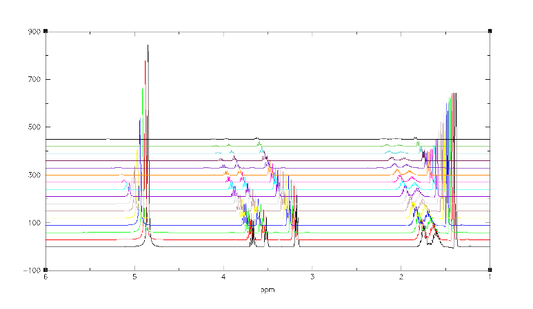
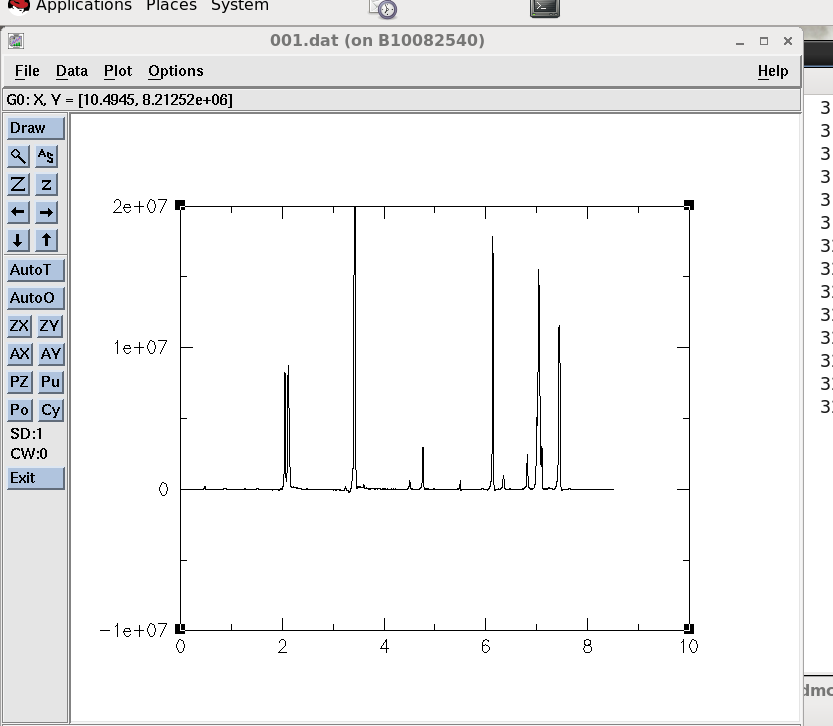
The dir should be populated with 600 1D files in XY text format. To list them ls and note they run from 001.dat to 600.dat. We can now use a graphing program to view the NMR spectra. I have flexible program xmgr installed on the dpx400.
xmgr - XMGR graphics plotter

eg) to view the first 1D file - xmgr 001.dat

We are now ready to edit the peak list file man.xpk such that we integrate all peaks of interest. Note that you can use xmgr to read off the ppm values by simply hovering the cursor between the ranges of the peaks you would like to integrate. Now manually edit the man.xpk file:

gedit man.xpk
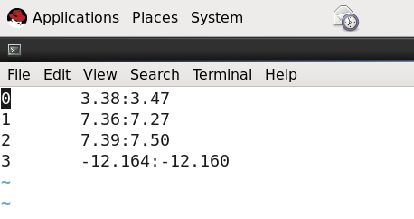
edit in all the peaks you'd like to integrate. It is ok to include the baseline as well as these are just zero's.
the order doesn't matter and negative values are OK too.

The simple peak list man.xpk format:

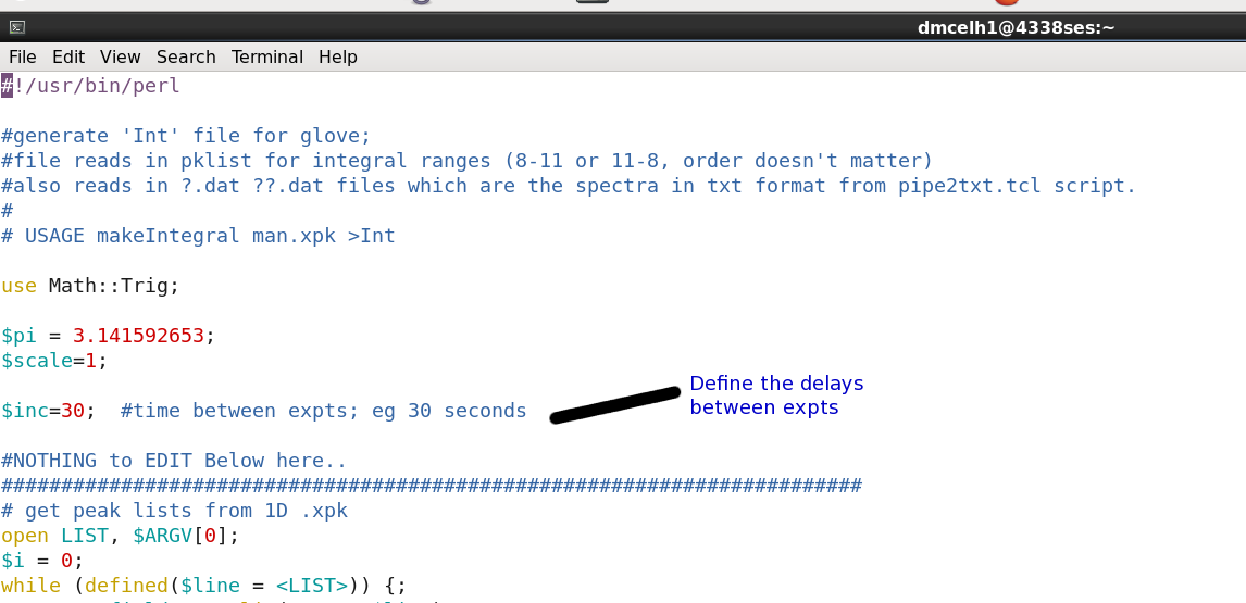
Next step is to run the integration routine. First define the delays here gedit mkxcel.pl

Then run:

./go_integral
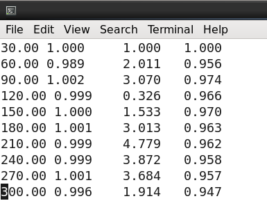
'excel.txt' file is generated and contains the integrals as X Y0 Y1 Y2 etc format.
where X=the defined delays btw expts; and Y0 is peak0, Y1 is peak1.. from man.xpk.
Please look inside 'go_integral' file to see what is occurring.

Here is what the output file 'excel.txt' looks like:

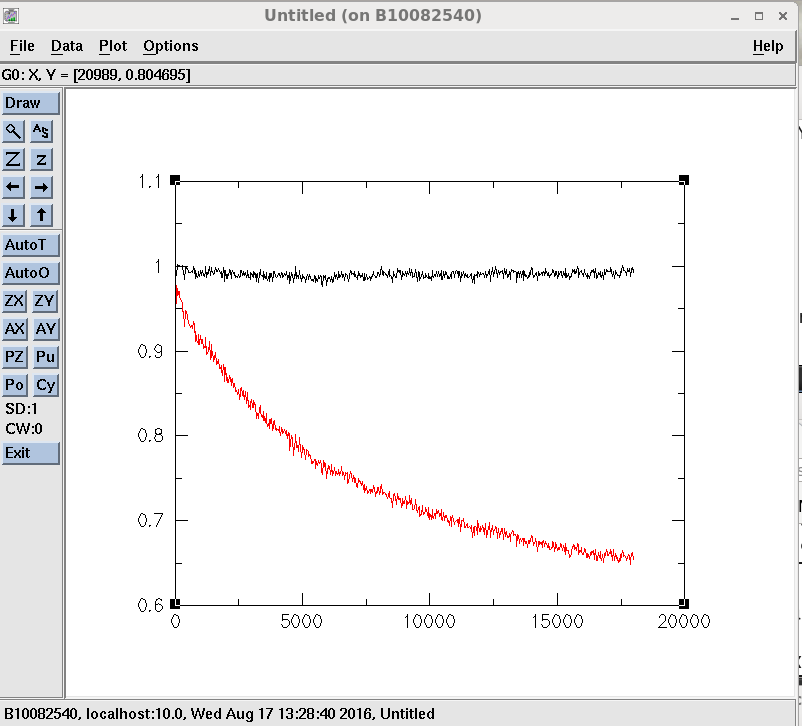
Note the first points are normalized to one. To plot 'block' data in xmgr try:

xmgr -block excel.txt -bxy 1:2 -bxy 1:4

Where we can see that peak0 in man.xpk doesn't decay and peak2 does. Peak0 could be used as a control.

Making Stacked Plots

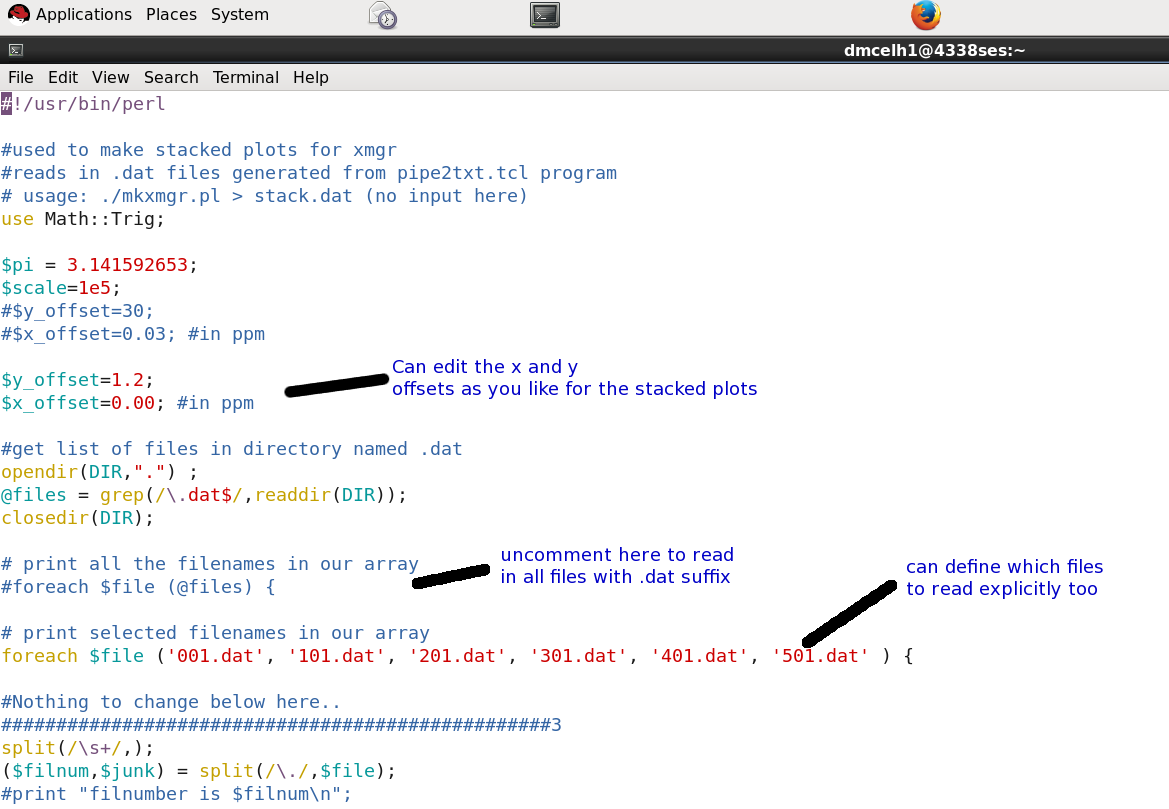
Generating stacked plots is trivial now with the use of the 'mkxmgr.pl' script.
eg) to define the X and Y offsets gedit mkxmgr.pl

Then create a file to read into xmgr by:

./mkxmgr.pl > stack.plot
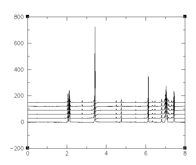
xmgr stack.plot

And XMGR plots:

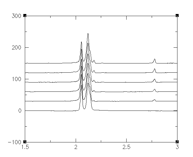
Can zoom into a region:

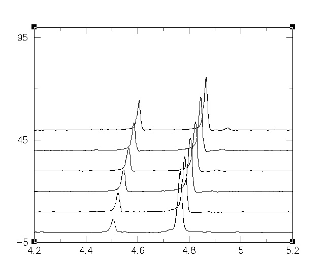
Adding a bit of X-offset too:

Some quick notes on xmgr plotting thru the pulldowns:

to flip x-axis data - graph operations - flip axes
Double click in plot window to change coloring, linewidths etc
See link for detailed info: xmgr - XMGR graphics plotter

Data Fitting with Glove

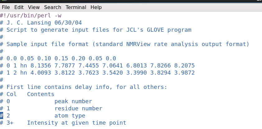
Upon running the integration routine an additional file named 'Int' was also generated. This contains the Delays and Intensities needed to run the fitting routine. In this cae I just used a 3 parameter exponential decay with 100 Monte Carlo simultations for error analysis. More on the software can be found at: GLOVE_paper

Also a tar ball of documents: More_notes

The format of 'Int' file:

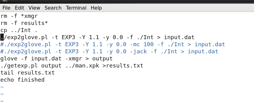
A directory w/the scripts was generated previously. Just type cd glove and look in the 'go_glove' script.

To launch the fitting routing ./go_glove
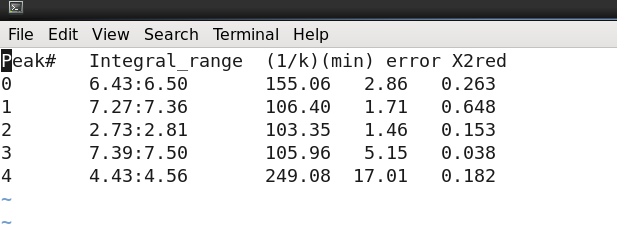
There are a few additonal examples of simultation with Jack-Knife and Monte-Carlo as well. The fitting results are piped into 'results.txt'

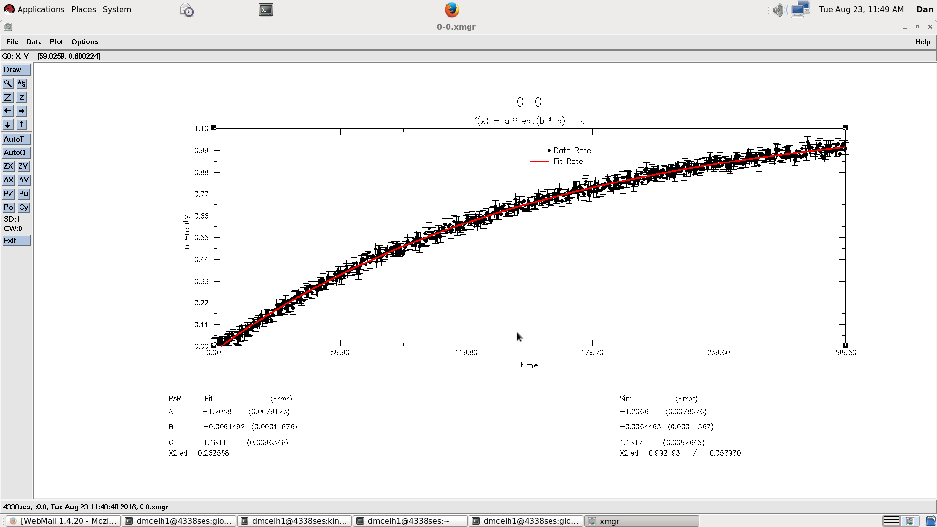
Lastly XMGR plots have been generated for each peak. To view the contents xmgr 0-0.xmgr etc