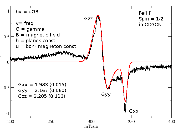
TABLE OF CONTENTS

Introduction
Open Matlab
The Fitting Script
Appendix

Introduction

This tutorial is a quick overview on how to run EasySpin using a simple Matlab script. The example is a simulation of published work regarding the g-tensor of Fe(III).

It is highly recommended to follow the EasySpin youtube videos first as they are a far better resource:

• EasySpin_Youtube - Excellent YouTube videos regarding Matlab/EasySpin

Software used:

1. CentOS 7 - My Linux OS
2. Matlab - Download Matlab from UofI webstore if at UIC.
3. EasySpin - Free EPR simulator.

Go ahead and download and unzip a starting directory: tut.zip
which will be named easy_spin_tut_fe3

Look in Dir:

$ cd easy_spin_tut_fe3 
$ ls
fe_fit_2.m  intermediate.dat  pathdef.m

Here you can see we have a few files:

• fe_fit_2.m - EasySpin matlab file
• intermediate.dat - The X/Y formatted EPR spectrum
• pathdef.m - Matlab path definitions.

Note ".m" suffix is for Matlab files. Please see EasySpin software install regarding setting the correct "pathdef.m" for your computer. This occurs automatically upon install and configuration.

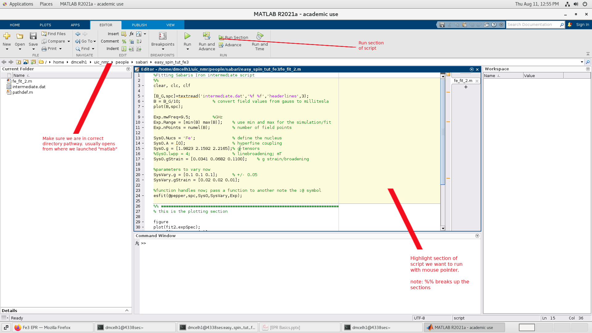
Open Matlab

$ matlab

Note we use the "Run Section" instead of "Run" button.
The software interface looks like:


Before using "Run section" we will see below.
The program loaded our initial guesses to the g-tensors and their
distribution defined as gStrain. I believe
the gStrain is expressed as a Gaussian distribution of g-tensor values
due to slight molecular distortions (ligand distance variations etc) within the sample.
This is an interesting result describing the order of such ligands around the metal center.


After running the Nelder simplex algorithm we get a plot of
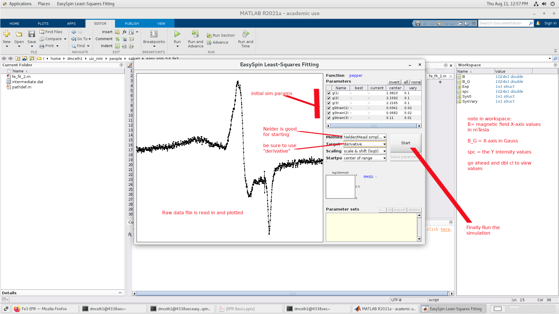
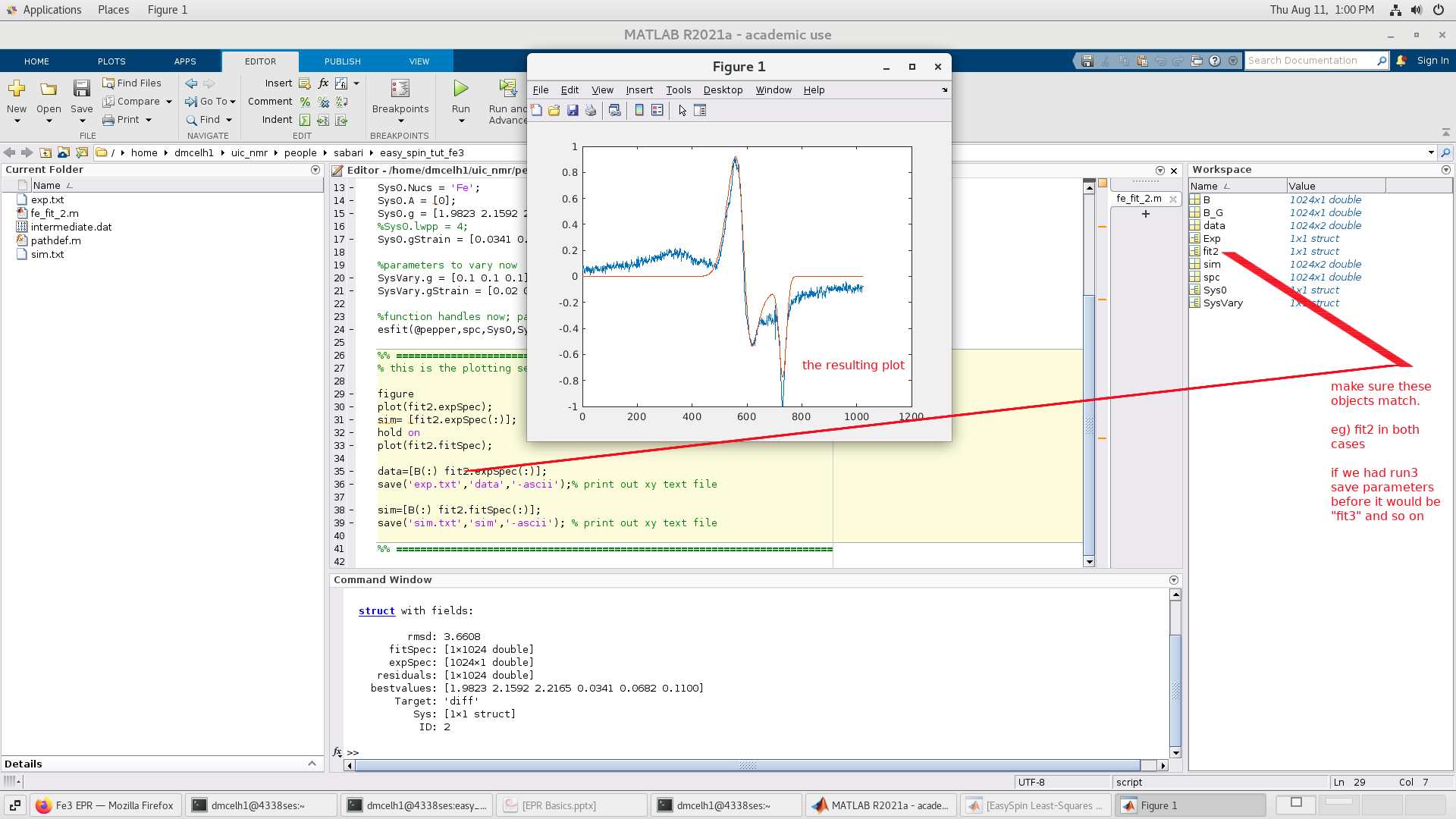
the simulation and experimental data. Now lets go one step further
and Minimize with the Levenberg/Marquardt algorithm:


OK great it converged fine and output the "bestvalues" in the
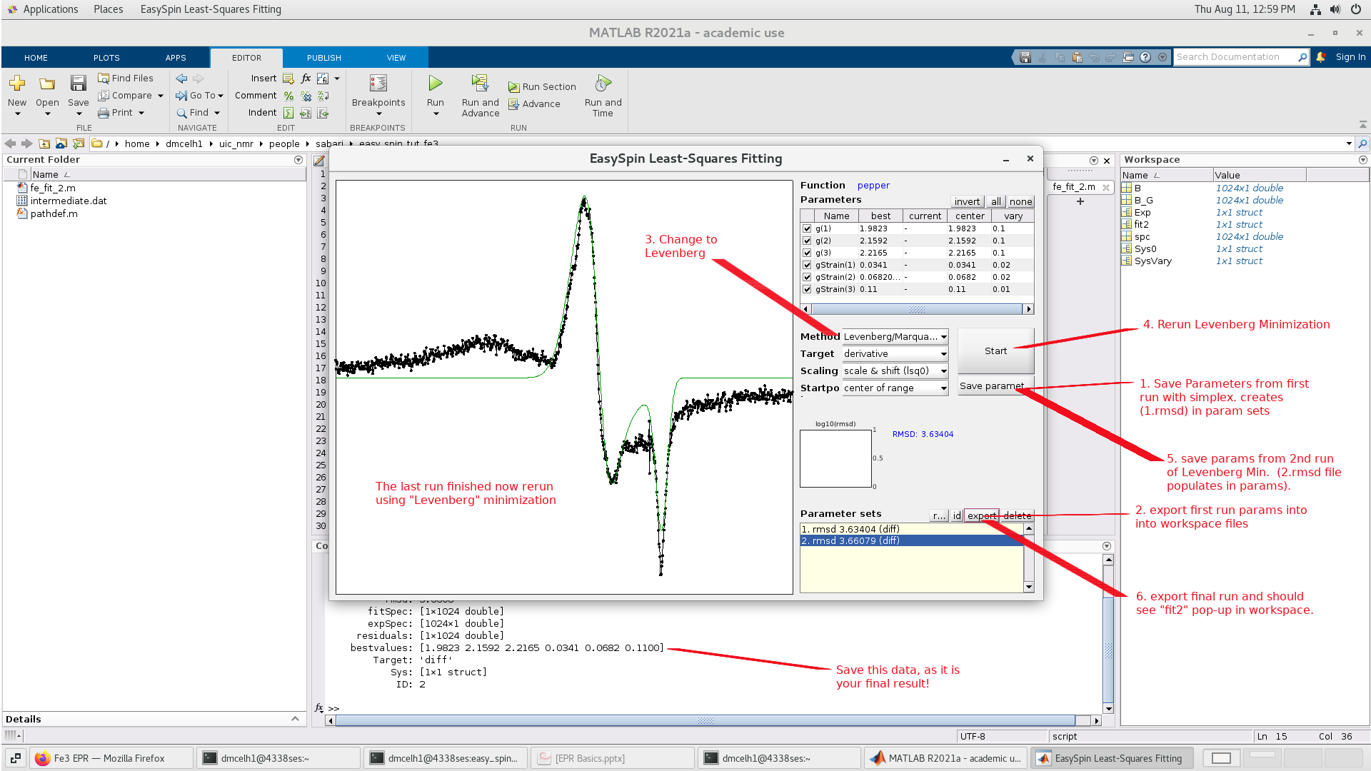
command window above. Cut and paste these values into a file for safe keeping.
Next we generate X/Y text file formats for the simulated and exptl data so we
can make plots in any program we choose. This is done in the "second" section of the
script defined by "%%":


If there are problems please be sure the file naming matches
within our .m script and the object eg) "fit2" in the Workspace:

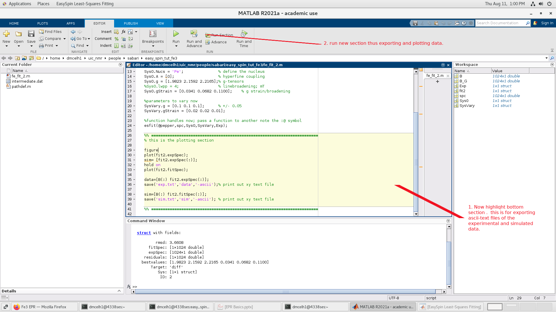
The resulting files are in text format:

• exp.txt - The original spectrum in ascii-text format
• sim.txt - The simultaed spectrum in ascii-text format

We are effectively done now with the simulation. However, I'd like to talk a bit more about the
matlab script used in the easyspin simulation.

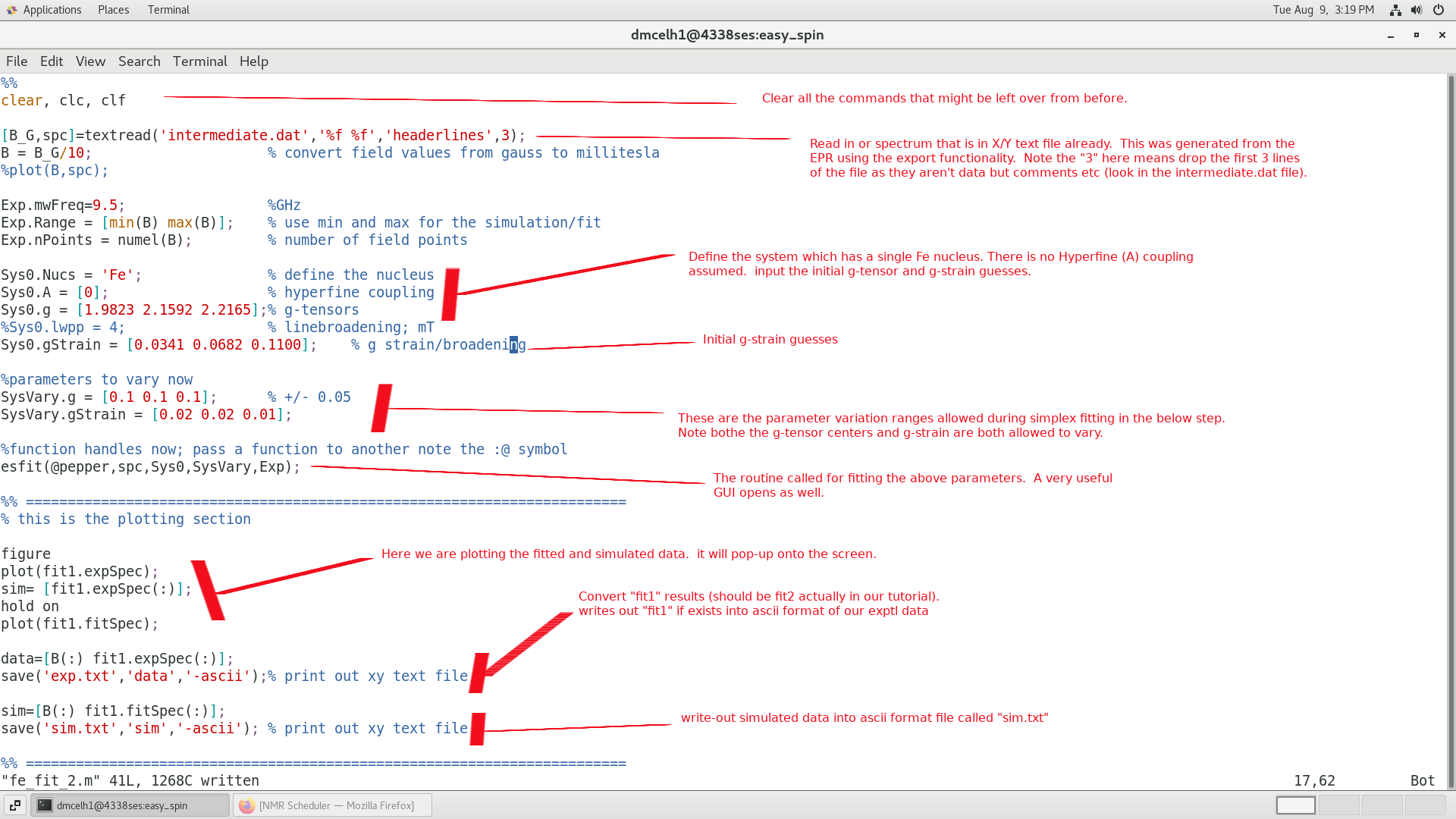
A closer look at the .m script

Please see the EasySpin documentation and tutorials for a better understanding. Below is a
very broad overview of how our script works.

Appendix Files:

All of the files for the tutorial are available here:
tut.zip