Convert DOSY spectra to text files and manually process
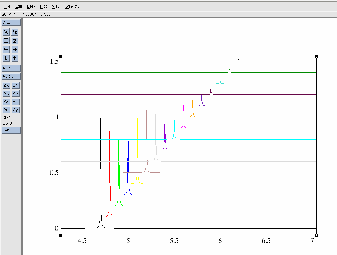
TABLE OF CONTENTS
IntroductionAcquire data in Topspin
Topspin Processing
Copy over Glove
Define the peaks to fit
Integrate and normalize peaks
Build the Glove input file
A closer look at the "input.dat
Fit a double exponential function
Appendix
Introduction
Fitting DOSY spectra can be somewhat of a black box. Here I try and add a little more control to the user in fitting the data through the use of text files, PERL scripts and the data fitting program GLOVE. Using software such as Topspin and MNova are still probably a better way to go, but this method here will allow for more robust fitting and error analysis of integrated peaks of interest using either "Jack Knife" or "Monte Carlo" simulations.Software used:
- CentOS 7 - The Linux OS which is free
- Topspin3.6.5 - Bruker NMR software
- GLOVE2 - Data fitting software
- PERL - A useful computer language for handling text files etc.
- XMGRACE - Graphical plotter also known as XMGR or Grace
*The above programs should all work in the Linux and MacOS environments.
The first part of our tutorial is directed towards people with access to our PC at UIC. Outside users can find the files at the bottom of this page however Appendix
DOSY_Manual -- Bruker manual for DOSY DOSY_Review -- A must read
Acquire Data
I like to use macros to load the DOSY experiments. Below is an example starting from Brukers default DOSY parameter set.
- macro: dosy.txi -- DOSY without water suppression pulprog Or for the case with water suppression:
- macro: dosy_es.txi -- DOSY with 3-9-19 water suppression. pulprog
Please be sure to correct the power levels in the "getprosol" statement for your machine. Also the last line in the macro includes an XAU call that sets up the DOSY gradient stepping from 5 to 95% in 16 steps. More info on this can be found in the Bruker manual above.
Topspin Processing
After acquiring the DOSY data process with:
- xf2 -- Fourier transform in 2nd dimension only
- manually phase the peaks; I leave it to the reader..
- abs2 -- Baseline correction in F2 only
- 2dtxt -- convert the spectra into a 2D file called "2d.txt". There are usually 16 1D spectra, but can be whatever.
The "2d.txt" file is saved in the pdata directory in the experiments file name. eg) my folder name is "dosy_water" and using a shell I find it in:
$ pwd
/opt/topspin3.5pl7/data/dan/dosy_water/3/pdata
$ ls
1  10  11  12  13  14  15  16  17  2  2d.txt  3  4  5  6  7  8  9
To view lets use the "xmgrace" software:
$ xmgrace ./2d.txt
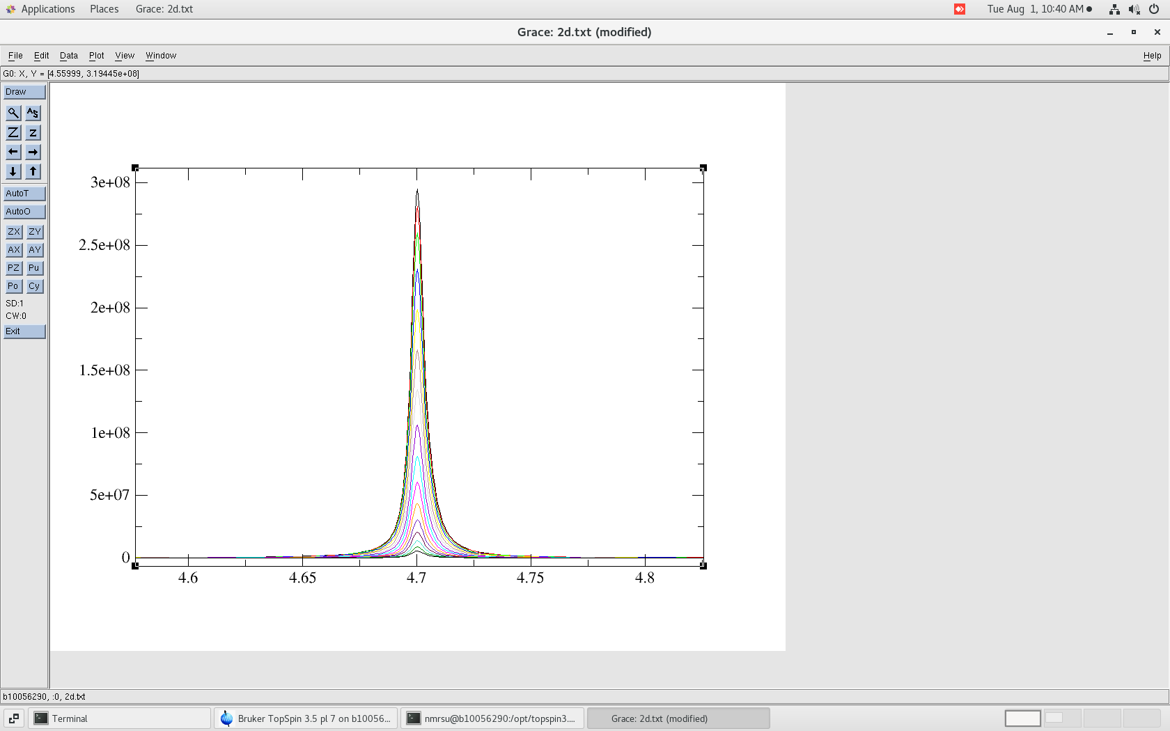
The resulting 2d.txt file looks like:
- 2d.txt - The ASCII/TEXT file
Note the "&" separation between each 1D spectrum. Also, be sure that the baseline looks correct as this can be a problem in DOSY data. That is the baseline should be centered about zero.
Copy over Glove
Lets copy over some Glove processing directories into the pdata directory as well. On our NMRs at UIC I leave some in /opt/dosy/ eg):
$ ls /opt/dosy
dosy_sim  glove_dosy  glove_dosy_global  old
And starting from our working processing directory:
$ pwd
/opt/topspin3.5pl7/data/dan/dosy_water/3/pdata
$ ls
1  10  11  12  13  14  15  16  17  2  2d.txt  3  4  5  6  7  8  9
$ cp -r /opt/dosy/glove* .
$ ls
1  10  11  12  13  14  15  16  17  2  2d.txt  3  4  5  6  7  8  9  glove_dosy  glove_dosy_global
The "glove_dosy" directory is for fitting each peak individually. The "glove_dosy_global" directory is for fitting all peaks to the same diffusion rate (more on this later).
Define peaks to fit
We will manually input the peak list ranges that will be integrated and later fitted to a Gaussian function. eg)
$ cd glove_dosy
$ pwd
/opt/topspin3.5pl7/data/dan/dosy_water/3/pdata/glove_dosy
$ ls
data_fit data_fit_2  get2dtxt_stacks.pl  go  go_xmgr  integrals.txt  mkIntegral.pl  peak.list  readme.txt
And having a look inside the peak.list file
$ more ./peak.list
0	4.60:4.80
1	4.52:4.91
We've basically defined two integral ranges for the same peak. The 1st column is the "peak number" The 2nd column is the "peak integral range" separated by a ":" To define additional peaks we could use the xmgrace plot and edit the "peak.list" using "gedit" or "vim". eg)
$ gedit peak.list
Integrate and normalize peak intensities
Having picked the peaks we can integrate each one now. The mkIntegral.pl script will integrate and normalize each peak to max intensity of unity. eg) To launch use the go script:
$ more ./go
rm -f ./Int
cp ../2d.txt .
#
./mkIntegral.pl peak.list 2d.txt
tail Int
$ ./go
 0  0  HN 1.00000 0.95338 0.88229 0.78364 0.67453 0.56388 0.45715 0.36004 0.27540 0.20454 0.14737 0.10306 0.06989 0.04600 0.02933 0.01820
 1  1  HN 1.00000 0.95344 0.88229 0.78354 0.67437 0.56368 0.45702 0.35990 0.27535 0.20449 0.14734 0.10307 0.06992 0.04603 0.02935 0.01825
mkIntegral.pl - The integration routine
The file Int is automatically generated (above) and the first column is the corresponding peak number from the peak.list file.
Build the Glove input file
We would like to generate a file called input.dat which glove reads.
$ pwd
/opt/topspin3.5pl7/data/dan/dosy_water/3/pdata/glove_dosy
$ cd data_fit
$ ls
clean         exp2glove_fixed.pl  getdosy.pl  go_plot  header          mk_dosy_sim.pl  plot.pdf    results.agr
exp2glove.pl  getdosy             go          gotemp   mk_dosy_int.pl  plot.bfile      readme.txt  xmgr.results
Annotations to the go script here:
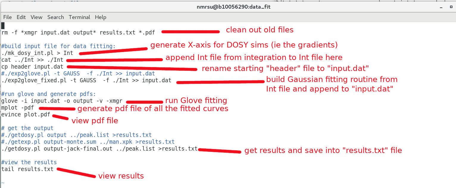
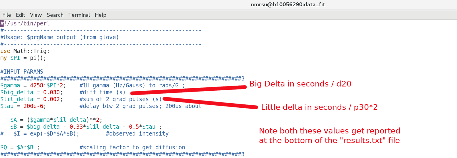
Make sure the mk_dosy_int.pl script matches your input parameters
mk_dosy_int.pl - This is used to build the effective applied gradients. Note this script basically reproduces the files the bruker command xau dosy 5 95 16 l y y builds upon execution. Things to check:- p_low -- lowest percent of gradient pulse (eg 5)
- p_highest -- lowest percent of gradient pulse (eg 95)
- G_probe -- Bruker probes are typically 5.35 G/cm/A or 0.0535 G/m/A
- I_max -- Bruker probes are typically 10 Amps max current
- scale -- This is the integral of the applied gradient pulse.
- -- A square pulse integrates to 1.0
- -- A sine lobe pulse integrates to 0.63
- -- A smoothed square pulse integrates to 0.90
Run the go script and simulate the data:
$ ./go
-------------------------------------------------------------------------
  METHOD (set ,       #/  total)          X2/DoF           | best X2/DoF
-------------------------------------------------------------------------
0.INIT   (   2,       1/      1)                1204.88    | 1204.88
1.RANDOM (   2,     500/    500)  25.005     -> 0.0692531  | 0.0692531
2.MCMIN  (   2,      99/    100)  349.71     -> 0.069253   | 0.069253
3.MCMIN  (   2,     100/    100)  173.4      -> 0.069253   | 0.069253
4.MCMIN  (   2,     100/    100)  319.24     -> 0.069253   | 0.069253
5.MCMIN  (   2,      99/    100)  279.33     -> 0.069253   | 0.069253
6.ONEEX  (   2,       1/      1)  0.069253   -> 0.069253   | 0.069253

# Jackknife simulation #1/32 (0-0 #1/16)
-------------------------------------------------------------------------
  METHOD (set ,       #/  total)          X2/DoF           | best X2/DoF
.
.
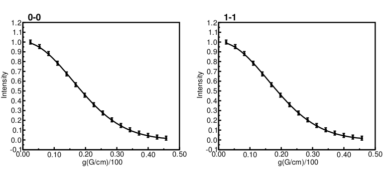
A somewhat verbose output is displayed showing the multiple minimization steps and the one exchange. See the "glove" manuscript for more detail. Upon completion a few files of interest are generated:
- results.txt -- the diffusion rates and errors/Chi squared are given
- plot.pdf -- each curve fit is piped into a clean pdf for viewing
- output-jack-final.out -- Results from the Jack-Knife simulations
- 0-0.xmgr -- Additional plots in XMGRACE format
The resulting plot file plot.pdf
And having a closer look at the results.txt file:
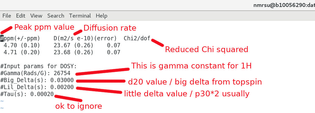
Be sure the getdosy.pl script above has the proper input parameters regarding Big Delta / Little Delta used in the NMR experiment. The Tau delay can largely be ignored if you like. eg):
$ gedit getdosy.pl
And that is basically it for fitting a DOSY curve to a 3 Parameter Gaussian exponential. Below we'll have a closer look at the input files and the format.
A closer look at the input.dat file
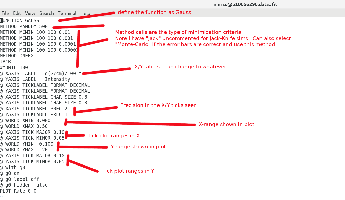
The input.dat file is a combination of a "header" and "exp2glove_fixed.pl output" files. The header defines the fit type, labels, ticks etc which can all be changed by the user. The exp2glove_fixed.pl script reads in the Int and generates the data in a format which can be read by the Glove software. eg) the header
and the data part : data
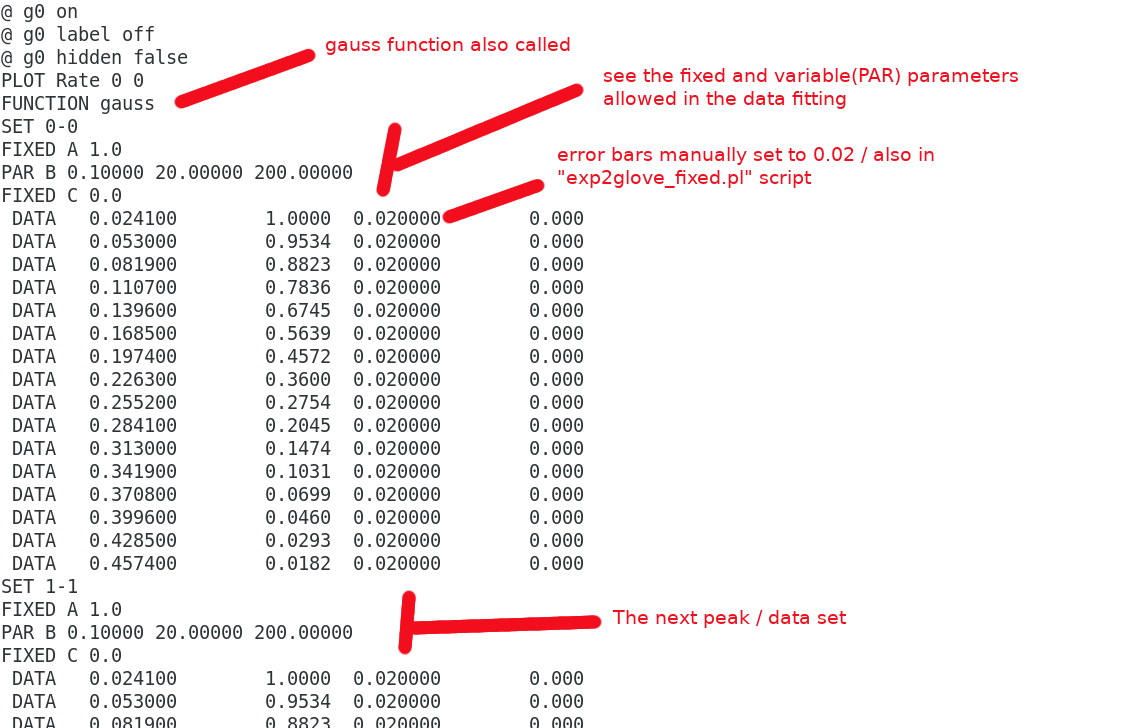
Lastly everything combined forming the input.dat : input.dat
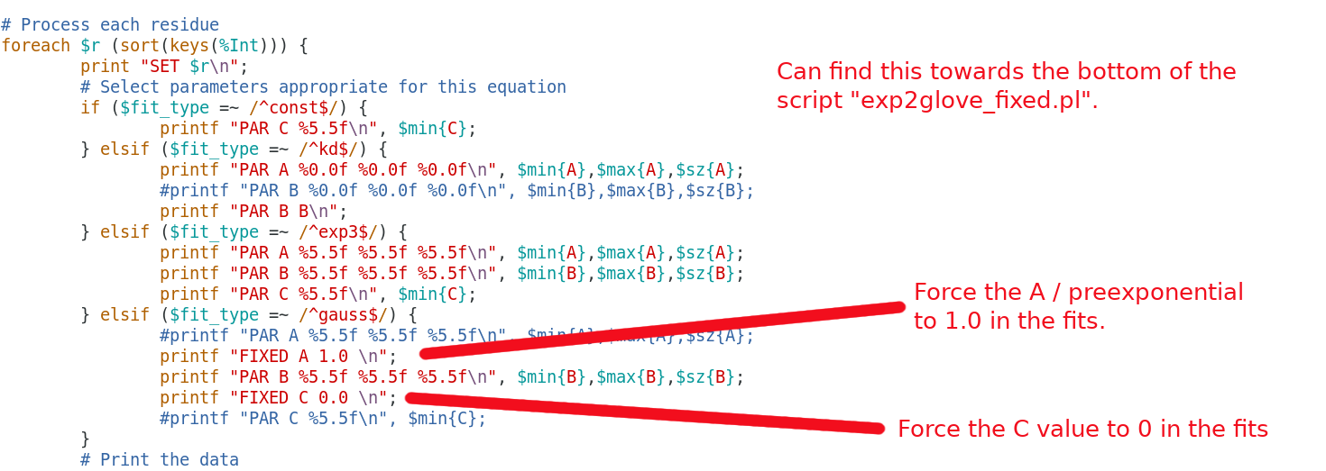
If you'd like to change the Fixed input values that is easily done just be editing the exp2glove_fixed.pl. eg):
$ gedit exp2glove_fixed.pl
Fit a double exponential
It is is often the case that a diffusion curve decays in a multi exponenital fashion. Lets try and fit our data and compare the Chi square from the mono to the double exponential. If the ratio of mono/double > 2 it is statistically valid then to use the more complex function. If it is less than two go with the simpler (mono-exponential) fitting. Lets try and fit with this equation:

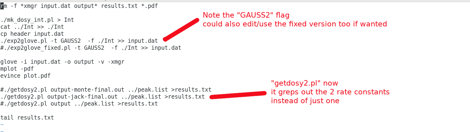
In glove the function is called gauss2 and the prexpontial A = 0.0 to 0.5 and the other is forced between C=0.5 to 1.0 use the directory data_fit_2
$ pwd
/opt/topspin3.5pl7/data/dan/dosy_water/3/pdata/glove_dosy/data_fit_2
$ gedit go
$ ./go
-------------------------------------------------------------------------
  METHOD (set ,       #/  total)          X2/DoF           | best X2/DoF
-------------------------------------------------------------------------
0.INIT   (   2,       1/      1)                408.295    | 408.295
1.RANDOM (   2,     500/    500)  51.2042    -> 0.00512359 | 0.00258025
2.MCMIN  (   2,       4/    100)  334.42     -> 0.0051236  | 0.0025802 2
.
$ pwd
/opt/dosy/glove_dosy/data_fit_2
$ more ./results.txt ../data_fit/results.txt
::::::::::::::
results.txt
::::::::::::::
#ppm(+/-ppm)	D(m2/s e-10)(error)  Chi2/dof
 4.70 (0.10)	51.01 (4.39)	22.22 (0.12)	0.003
 4.71 (0.20)	50.76 (4.29)	22.20 (0.12)	0.003

#Input params for DOSY:
#Gamma(Rads/G): 26754
#Big_Delta(s): 0.03000
#Lil_Delta(s): 0.00200
#Tau(s): 0.00020
::::::::::::::
../data_fit/results.txt
::::::::::::::
#ppm(+/-ppm)	D(m2/s e-10)(error)  Chi2/dof
 4.70 (0.10)	23.67 (0.26)	0.069
 4.71 (0.20)	23.68 (0.26)	0.070

#Input params for DOSY:
#Gamma(Rads/G): 26754
#Big_Delta(s): 0.03000
#Lil_Delta(s): 0.00200
#Tau(s): 0.00020
The chi square improves dramatically with mono/double being 0.070/0.003 = 23.3 Consequently the more complex double function would be justified. It is interesting the prexponentials are also A=0.11 and C=0.89 This sample is 90/10 H2O/D2O so the fitting is picking up on the heavy water contribution to the 2 diffusion rates 51e-10 versus 22e-10 m2/s